How to use idaifieldR: Detailed Workflow • idaifieldR

idaifieldR imports data from iDAI.field / Field Desktop directly into R via the CouchDB API. This eliminates the need for CSV exports and allows scripts to be re-run and updated whenever the database changes.

Installation

idaifieldR is not yet on CRAN. Install it from GitHub using remotes:

remotes::install_github("lsteinmann/idaifieldR")
library(idaifieldR)

Connecting and Loading Data

To follow along with this tutorial, load the test dataset bundled with the package into a new Field Desktop project called rtest. The import file is located at inst/testdata/rtest.jsonl on GitHub.

Create a connection object with connect_idaifield():

conn <- connect_idaifield(pwd = "hallo", project = "rtest")

You can also ping the database to see if the connection succeeds:

idf_ping(conn)

If Field Desktop is running on the same computer, the serverip argument can be left at its default ("localhost"). The pwd argument is the password set in Field Desktop under Tools > Settings > Your password.

Load the complete project database into R:

idaifield_test_docs <- get_idaifield_docs(connection = conn)

The result is a named list of class idaifield_docs — one element per resource, named by identifier, reflecting the original JSON structure. Loading the whole database at once can be slow and memory-intensive for large projects; see the Queries section for a more targeted approach.

Building an Index

The index maps UUIDs to human-readable identifiers and is used by simplify_idaifield() to make relations readable. Generate it with get_field_index():

index <- get_field_index(conn, verbose = TRUE, gather_trenches = TRUE)

With verbose = TRUE the index also includes the shortDescription. With gather_trenches = TRUE the Place column is added, which contains the nearest Place-category resource (if any). Use head(index) to inspect it, or plot a quick overview of the dataset:

index |>
  ggplot(aes(y = Place, fill = category)) +
  geom_bar() +
  labs(title = "Resources by context and category", y = "Place", x = "Count")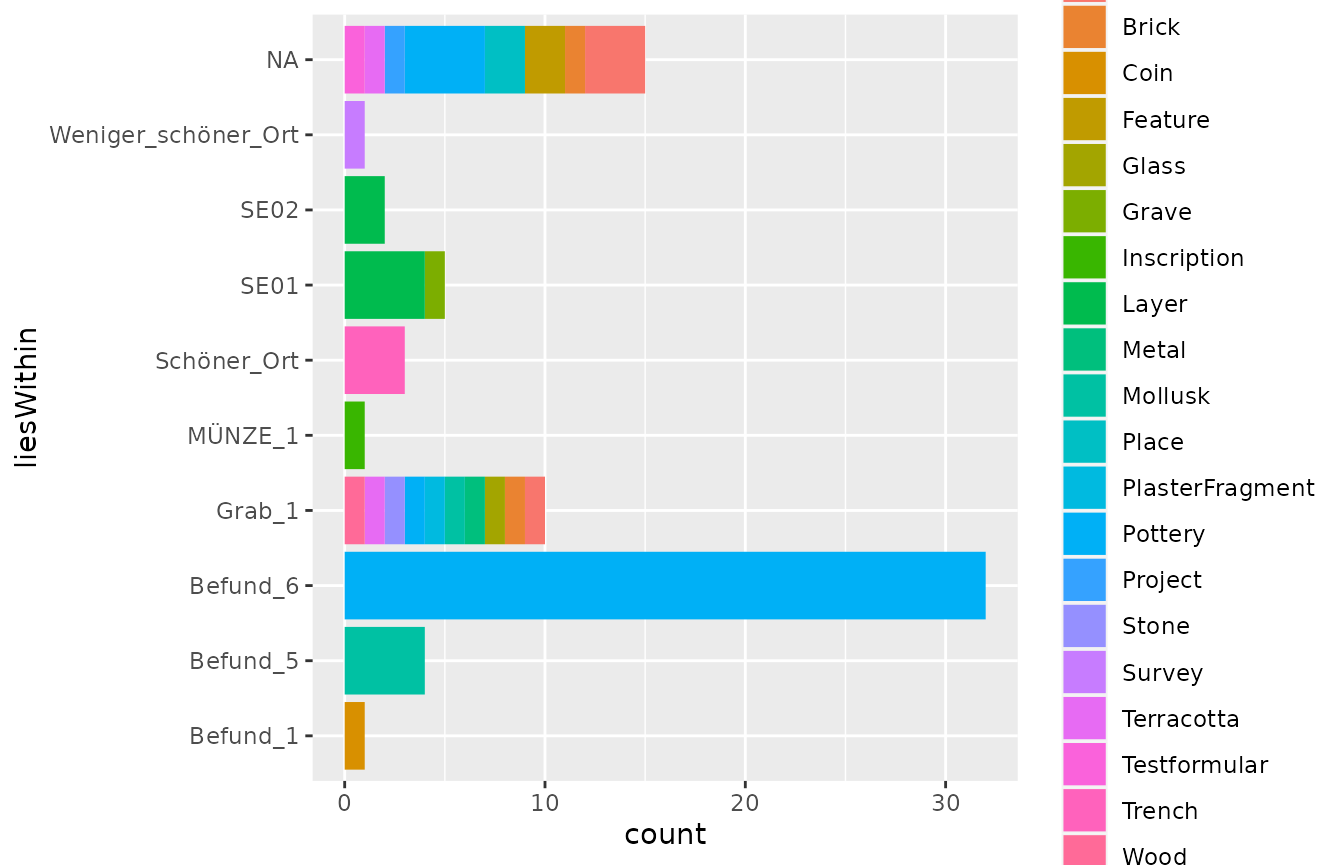

Unnesting (Optional)

get_idaifield_docs() returns the raw nested structure as it comes from the API, containing the complete revision history for each resource. You can reduce it to the resource level with maybe_unnest_docs():

idaifield_test_resources <- maybe_unnest_docs(idaifield_test_docs)

This step is optional — all idaifieldR functions handle both idaifield_docs and idaifield_resources lists. The unnested version takes up less memory and is easier to browse in RStudio.

Simplifying the Data

simplify_idaifield() transforms the nested list structure into something more R-friendly:

Relations are flattened into named vectors with a relation.-prefix (e.g. relation.liesWithin)
UUIDs in relations are replaced with human-readable identifiers
Geometry is kept as a GeoJSON string if keep_geometry = TRUE
Single level lists are flattened to vectore, but more complex fields are preserved as-is.

You need to supply the index of the complete project database here, even if you are working with a subset — it is used as a lookup table for UUID replacement. You also need to supply the project config:

config <- get_configuration(conn)

idaifield_test_simple <- simplify_idaifield(
  idaifield_test_resources,
  index        = index,
  config       = config,
  keep_geometry = TRUE
)

The result has class idaifield_simple. The connection and project name are stored as attributes and carried through for later use. Check them with attributes(idaifield_test_simple).

Selecting Resources

Use idf_select_by() to filter the simplified list by any field:

pottery <- idf_select_by(idaifield_test_simple, by = "category", value = "Pottery")

Queries

Alternatively, query the database directly instead of loading everything first. This is useful for large projects where you only need a small subset:

pottery_docs <- idf_query(conn, field = "category", value = "Pottery")

# Always supply the index of the complete database when simplifying a subset
pottery_simple <- simplify_idaifield(pottery_docs, index = index, config = config, keep_geometry = TRUE)

See also ?idf_index_query and ?idf_json_query for more targeted queries.

Converting to a Data Frame

Convert the simplified list to a matrix and then a data frame with idaifield_as_matrix():

pottery_df <- idaifield_as_matrix(pottery) |>
  as.data.frame()

From here, standard R and ggplot2 workflows apply:

pottery_df |>
  ggplot(aes(x = relation.liesWithin, fill = period.start)) +
  geom_bar() +
  labs(title = "Pottery by context and period",
       x = "Context", y = "Count") +
  theme(axis.text.x = element_text(angle = 45, hjust = 1))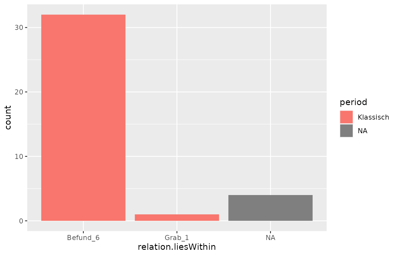

pottery_df |>
  ggplot(aes(x = vesselForm, fill = specificType)) +
  geom_bar() +
  labs(title = "Pottery by vessel form and type",
       x = "Vessel form", y = "Count") +
  theme(axis.text.x = element_text(angle = 45, hjust = 1))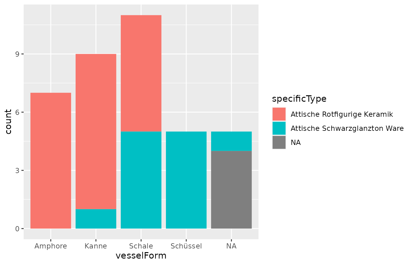

Geometry

Geometry is kept as a GeoJSON string when keep_geometry = TRUE in simplify_idaifield(). To convert to an sf object for spatial analysis:

library(sf)
geom <- sf::st_read(pottery_simple$Befund_6_KER_4$geometry)
plot(geom)

Please note that you will need to set the CRS manually.

Working with the Raw List

If the matrix format does not suit your analysis, work directly with the idaifield_resources or idaifield_simple list. Each element is a named list corresponding to one resource — extract fields directly, apply your own lapply() transformations, or use purrr to reshape the data as needed.